Terms and Definitions
Variable
Variables are any characteristic that are measured, controlled or manipulated 1 (e.g.: concentration, time).
Dependent variable
A variable which is measured or registered and is expected to be dependent on manipulation or experimental conditions 1 (e.g.: concentration in PK)
Independent variable
A variable which is manipulated or which is a predictor variable 1 (e.g: demographics)
Parameter
A parameter is a model coefficient relating dependent and independent variables. In PKPD these parameters relates to some mechanistic property of either the drug or biology. (e.g.: mean population clearance (CL), between subject variability of CL, CL in an individual).
Model
A model is a quantitative representation of the relationships among the entities in a system, often used to make predictions about the system.2
In the context of PKPD, a model is a mathematical form specifying the probability distribution of random variables representing observations (here drug concentrations and effect) in a subject-matter domain, and which may be the composition of several submodels (e.g.: one for PK, another for PD), including ones for the distribution of unobservable conceptual entities (e.g.: drug clearance in the population)3
Linear and Non-Linear Model
A Linear model can be function of the form
y =ƒƒ(x;β) = β0+β1•x1+ β2•x2+…
where
x denotes the vector of independent variables
β denotes the vector of model parameters.
and in which
- Each independent variable is multiplied by an unknown parameter,
- There is at most one unknown parameter with no corresponding independent variable, and
- All of the individual terms are summed to produce the final function value.
A nonlinear model can be a function of the form
y = ƒ(x;β) = β0+β0• β1•x1
in which
- The functional part of the model is not linear with respect to the unknown parameters β0,β1…
One way to determine if a model is linear or nonlinear in the model parameters is to compute partial derivatives with respect to each of the parameters in the model.
The model is linear if none of the partial derivatives involve model parameters
The model is nonlinear if the partial derivative with respect to one parameter involve another parameter.
Fixed Effect Parameter
Fixed effect parameters are population parameters, which define the average value for a parameter in a population and/or the average relationship between measurable patient factors (creatinine clearance) and pharmacokinetic parameters (renal clearance).4
Typical value of a parameter is the average parameter value at specific covariate value. (e.g.: 72L/hr/70kg). The typical value equals the average population value when no covariates are used.
Random Effect Parameters
Random effect parameters are population parameters, which quantify random (unknown) variation. Random effects can be subdivided into:
- Between subject variability (BSV) - A measure of unexplained random differences between individuals. BSV is also called as inter-individual variability.
- Residual variability - A measure of remaining unexplained variability when all other sources of variability has been accounted for. It includes measurement error and model specification errors. Generally, statistical literature refers to this as within subject variability (WSV) or intra-individual variability.
- Between occasion variability (BOV) - A measure of unexplained random differences in an individual between different occasions.
Mixed Effects Modeling
Population analysis (PK or PD) is usually performed by the mixed effects modeling approach. A mixed effect model mixes the effects of random quantities (BSV,WSV) and fixed effects (age, weight, creatinine clearance) on the observations i.e., plasma concentrations, allowing these influences to be simultaneously quantified.4
Nonlinear mixed effects modeling involves approximation during estimation. Linear mixed effects modeling does not suffer from these approximations. Linear models can be identified using the partial derivative method and linear mixed effects modeling can be used when needed.
Structural Model
The structural model is the deterministic part of a population model. A complete population PK / PD model usually constitutes of four structural and three statistical (error) models. The four structural models include: (1) PK model, (2), disease progression model, (3) PD model and (4) covariate (or prognostic factor) model. The parameters of these models are called as 'fixed effects'. Examples of fixed effects include the typical value of systemic clearance in a 70 kg person and the mean potency of the drug. (e.g.: a two - compartment model or an Emax model).
Random Effect Model
Random effect models are between subject variability (BSV) model, residual variability model and between occasion variability (BOV) model.
- Between subject variability (BSV) model: BSV refers to the random variability between individuals. Individual kinetic parameters are modeled as functions of population means and individual random deviations (η). η's are assumed to be identically, independently distributed with N(0, ω2).
- Residual variability model: A residual variability model includes intra-individual error, measurement error and any model misspecification error and represents the uncertainty in the relationship between the plasma concentrations predicted by the model and the observed concentration.
- Between occasion variability (BOV) model: BOV includes the variability in the pharmacokinetic parameters within an individual between occasions. BOV is modeled by lumping it in the residual variability in certain softwares (e.g.: NONMEM)
Population Pharmacokinetics And Pharmacodynamics
Population pharmacokinetics is the study of the sources and correlates of variability in drug concentrations and effects among individuals who are the target population receiving clinically relevant doses of a drug of interest. (As adapted from FDA guidance)5
Mostly the phrase population analysis is being used to refer to one-stage analysis when it is equally applicable to standard two stage approach.
Maximum Likelihood Approach
A maximum likelihood approach finds that estimate of a parameter, which maximizes the probability of observing the data given a specific model for the data.6
Objective Function Value
An objective function value is the sum of squared deviations between the predictions and the observations. Depending upon the estimation methods (Ordinary least squares (OLS), Extended least squares (ELS), Weighted least squares (WLS)) the objective function is appropriately weighted.
In NONMEM, The objective function is not a sum of squares, it is -2 times the log of the likelihood. The likelihood, in simple normal problems is a sum of squares.
Optimization Procedure
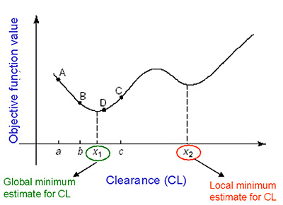
Optimization is a process of finding that estimate of a parameter, that maximizes or minimizes a given function.7 For e.g.: In a maximum likelihood approach, it is that value of the parameter which maximizes the objective function value. Different softwares use different optimization algorithms (Newton-Raphson, Simplex, Nelder-mead, E-M algorithm etc.,) Optimization invariably proceeds by iteration. Starting from an approximate trial solution, a useful algorithm will gradually refine the working estimate until a predetermined level of precision has been reached. If the function is smooth, an optimization algorithm can be expected to converge to a maxima or minima when given a sufficiently good starting value. A good starting value is one of the keys to success.
The diagram below shows how an optimization algorithm (golden search method) converge to either a local minima or global minima of a function.

Log-Likelihood Ratio
When the objective function value is computed as -2 times the log of the likelihood, competing nested models (covariate model and no covariate model) are compared by calculating the difference between their objective function value referred to as log-likelihood ratio. The log-likelihood ratio is assumed to be Chi-squared distributed. A difference in objective function value of 3.84 is considered to be significant at p < 0.05 with one degrees of freedom (difference of one parameter between the two nested models).
Point Estimate
A single numerical value used as an estimate of a population parameter. For e.g.: population mean. A point estimate does not provide any information about the inherent variability of the estimator.
Confidence Interval
An interval that estimates a population parameter within a range of possible values at a specified probability. The confidence interval reflect the uncertainty associated with the parameter estimate or in other words, the precision of a parameter estimate.
A 95% confidence interval for a population mean can be described in the following manner 9.When a clinical trial is repeated 100 times, and if we construct 100 confidence intervals out of those trials, 95 of those confidence intervals would contain the population mean and 5 of the intervals would not.
Caution: A 95% confidence interval of a mean is not to be defined as 95% of the population mean lie in the interval, nor 95% of the times the population mean is contained in the interval.
- Most mixed effects modeling softwares provide the asymptotic standard error's (S.E), which can be used to derive confidence intervals.
- These S.E's are estimated assuming the possible values are normally distributed, which may not be applicable to variances or Emax function. i.e., Maximum value for Emax = 1, a confidence interval greater than one does not make sense.
Maximum A Posteriori / Posthoc Estimates
The prior distribution of the parameters across a population and the actual data of the individual are used to obtain the posterior probability of individual parameter estimates. These estimates are called maximum a posteriori or posthoc estimates.
Simulation
Simulation is the use of the model to predict future outcomes, such as drug effect after an altered dosage regimen. Simulation can be broadly classified into deterministic and stochastic simulation. 8
- Deterministic simulation
These simulations are performed using a 'simulation model' , with no stochastic (statistical) sub models. They consider only typical values of the parameters and not the entire distribution of the model parameters. e.g.: role of dosage regimen in controlling pharmacodynamic responses.
- Stochastic simulation
These simulations are performed using a 'simulation model' with the stochastic sub-models. They consider the interpatient, inter occasion and/or residual variability. (e.g., evaluation of equivalence intervals of highly variable drugs)
Stochastic simulations can be classified into
- Parametric (Monte Carlo) simulations
These simulations are performed by resampling from one or more parametric distribution models, for e.g.: sampling the clearance of the drug given the mean and variance of a log normal distribution.
- Non-parametric simulations
Simulations are performed by resampling from sets of observed data, as opposed to using a distribution fitted to these data, for e.g.: sampling the clearance of a drug from a set of clearances using the bootstrap techniques.
- Parametric (Monte Carlo) simulations
Clinical Trial Designs
The most widely used clinical trial designs to evaluate effectiveness and safety of a drug are parallel, cross - over, and titration designs.
- Parallel
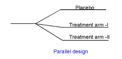
In a parallel design trial, patients are randomized into cohorts who receive one of the several treatments (control, dose 1, dose 2 or dose 3). ). Such a design will offer the population, rather than the individual, PK / PD characteristics. The advantage of such a design is the lack of confounding factors such as time (carry over effects) and design dependent outcomes. An illustration of parallel design is given below:

- Crossover
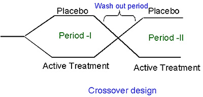
In a crossover design, each patient receives some (incomplete block) or all (complete block) of the treatments being studied.Therefore, a cross - over design is the most powerful design if deducing the individual concentration (or dose) - response curves is the ultimate aim. In a crossover design, three types of effects are evaluated. They are period effect (Period I vs Period II), Carry over effect and sequence effect (Placebo, active treatment or active treatment , placebo).The disadvantages of this approach are that of its longer trial duration, possible carry - over effects from previous doses and the need for sophisticated data analysis (nonlinear mixed effects modeling). An illustration of crossover design is provided below:

- Titration
The titration design ensures that the patients usually start at a relatively low dose and the dose is increased gradually until either no additional benefit is observed or dose - limiting toxicity occurs. This design closely resembles the clinical practice and the individual PK / PD characteristics can be obtained. The major disadvantage of this design is that of the possibility of an inverted U-shaped PK / PD relationship, as an artifact. The patients who are less sensitive to the drug need higher doses of the drug, making it appear as if the response decreases after a certain dose. Data analysis using conventional methods such as ANOVA fail and the use of sophisticated modeling techniques is required
Pharmacodynamic Terms
- Response: Response is any entity of a system that can or is measured. e.g.: Glucose concentration, forced expiratory volume.
- Effect: Effect is calculated as difference between the baseline response and maximum/minimum response. e.g.: % decrease in blood glucose concentration.
- Efficacy: The maximum effect that can be produced by a drug.
- Potency: A potency of the drug, is the dose at which 50% of maximum effect is attained.
- Effectiveness: Effectiveness is a simple 'yes' or 'no' answer to show that the drug works or not.
References
- Link to statistics glossary, Accessed March 20, 2005
- Definition for model, Accessed March 20, 2005
- Sheiner & Steimer, 2000,Pharmacokinetic/pharmacodynamic modeling in drug development. Annu Rev Pharmacol Toxicol. 2000;40:67-95
- Grasela TH, Sheiner LB., 'Pharmacostatistical modeling for observational data,' Journal of PK & Biopharm 1991: 19(3) (June Supplement):11S-23S
- Aarons, L., 'Population Pharmacokinetics: Theory and practice,' Br J Clin Pharmacol 1991; 32: 669-670
- Maximum likelihood, Accessed March 20,2005
- Optimization procedure
- Gobburu et al, 2001,Utilisation of pharmacokinetic-pharmacodynamic modelling and simulation in regulatory decision-making. Clin Pharmacokinet. 2001;40(12):883-92
- SB Tan, Introduction to Bayesian Methods for Medical Research. Ann Acad Med Singapore.2001;30:444-446
