Rational Modeling Process

1. Project Plan

All models are exploratory

The first step in the modeling process would be to develop a project plan.

It is important to identify the critical questions that are intended to be answered. For primary analysis in pivotal clinical trials, the modeling plan has to be mentioned a priori.

---

2. Preliminary Data Analysis

The main purpose is to get a general feel for the structural model. Preliminary data analysis can be performed by one or combination of the following methods.

A search of the literature could be done to obtain information of the drug under study, refer to previous studies of the compound or similar compounds and understand the biology of the disease etc.,

General feel about the data could be obtained by plotting the data from all the individuals or few representative individuals during preliminary model building process.

Pharmacokinetics (PK)

In the initial step of model building exercise a semilog plot of concentration versus time could help in answering the following questions.

1. What is the general trend in the data? When does Tmax occur?
2. Are there any implausibility in the data? ie., any outliers ar any unexpected data
3. How many disposition phases are observed in the semilog plot of concentration versus time? ie., Is the decline mono-exponential (one compartment) or multi-exponential (two compartment or more)
4. Are there any multiple peaks observed in the oral data? If so, the reasons could be explored.
5. Do the curves superimpose when the data are dose-normalized? ie., Plot of concentrations divided by dose administered versus time would reveal non-linearity if the curves do not superimpose.

Pharmacodynamics

A plot of effect versus concentration and a plot of response versus time could help in answering the following questions.

1. Does the effect versus concentration curve show hysteresis? ie., If there is anti-clockwise hysteresis then there is a delayed effect observed for the drug.
2. When does maximum repsonse (T_Rmax or T_Rmin) or minmum response occur occurs? Does it match the Tmax of PK? If yes, then the drug exhibits a direct effect. If not, then the drug might be eliciting an indirect effect. The indirect effect may be due to a distributional delay to the effect site. Alternatively, the drug might be affecting the formation and dissipation of response. A rational choice of model can only be made by considering plausible mechanism of action of the drug.

1. Where applicable, NCA should be conducted, provided linear pharmacokinetics is assumed. NCA cannot be performed on sparse data.
2. The summary statistics of the results should serve as reasonable initial estimates

---

Determination of Initial Model

• Preliminary data analysis would give an idea of the number of disposition phases for the drug or about the PD model.
• A simple structural model could be defined by NAD or by NPD approach. (NAD or NPD approach)

Structural model could be expressed in terms of primary PK or PD parameters, ie., clearances and volumes , rather than rate constants, as it would be easier to explore relationship between parameters and covariates like weight, sex, age or creatinine clearance.

1. Between subject variability (BSV) model

BSV models could be

• Additive (normal)
  • CL_i = CL_pop + η_CL where
  • CL = individual clearance
  • CL_pop = Population clearance
  • η_CL = random between subject variability
• Proportional
  • CL_i = CL_pop • (1 + η_CL)
• Exponential (log normal)
  • CL_i = CL_pop • exp(η_CL)

Given that all PK parameters are usually considered to be positive, they cannot arise from a normal distribution. The above lognormal distribution model implies that the distribution of individual clearances are skewed to the right which is a commonly observed feature of distributions of pharmacokinetic parameters.

Note: Proportional and exponential BSV models are indistinguishable when a First order estimation (FO) method (in NONMEM) is used because of the approximations involved.

Caution: Use of an exponential error model for PD parameters like slope (linear effect) or Emax is not possible.

2. Between occasion variability (BOV) model

BOV models can also be additive, proportional or exponential as explained above in BSV models. Random between occasion variability (Variance) is assumed to come from the same distribution for a parameter for all occasions inorder to reduce the number of parameters.

3. Residual variability or Within-subject variability (WSV) model

WSV (also called as intra-individual variability) includes intra-individual error, measurement error and any model misspecification error.

In order to choose the correct appropriate residual error model, it is essential to understand the concepts of weighting. Consider a typical calibration curve for an analytical method with three standards (1, 10 and 100 ng/mL). The standard deviations (determined using say 3 samples) of these concentrations could be similar or dependent on the concentrations. If the standard deviation is constant (see Figure 1 below) the variance is considered homoscedastic. However, if it is not then the variance is considered heteroscedastic (Figure 2). For HPLC methods, generally, the standard deviation is proportional to the sample concentration.

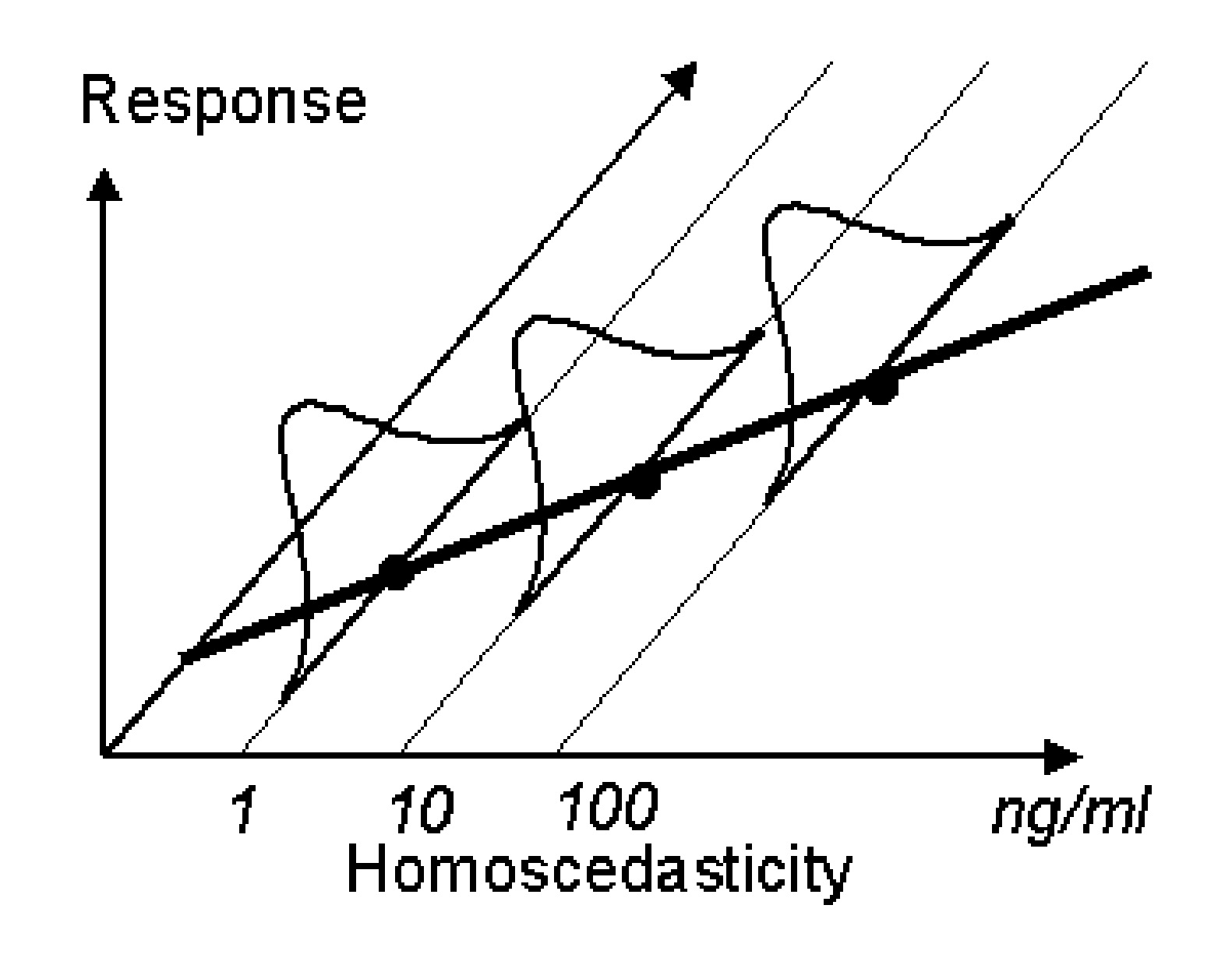
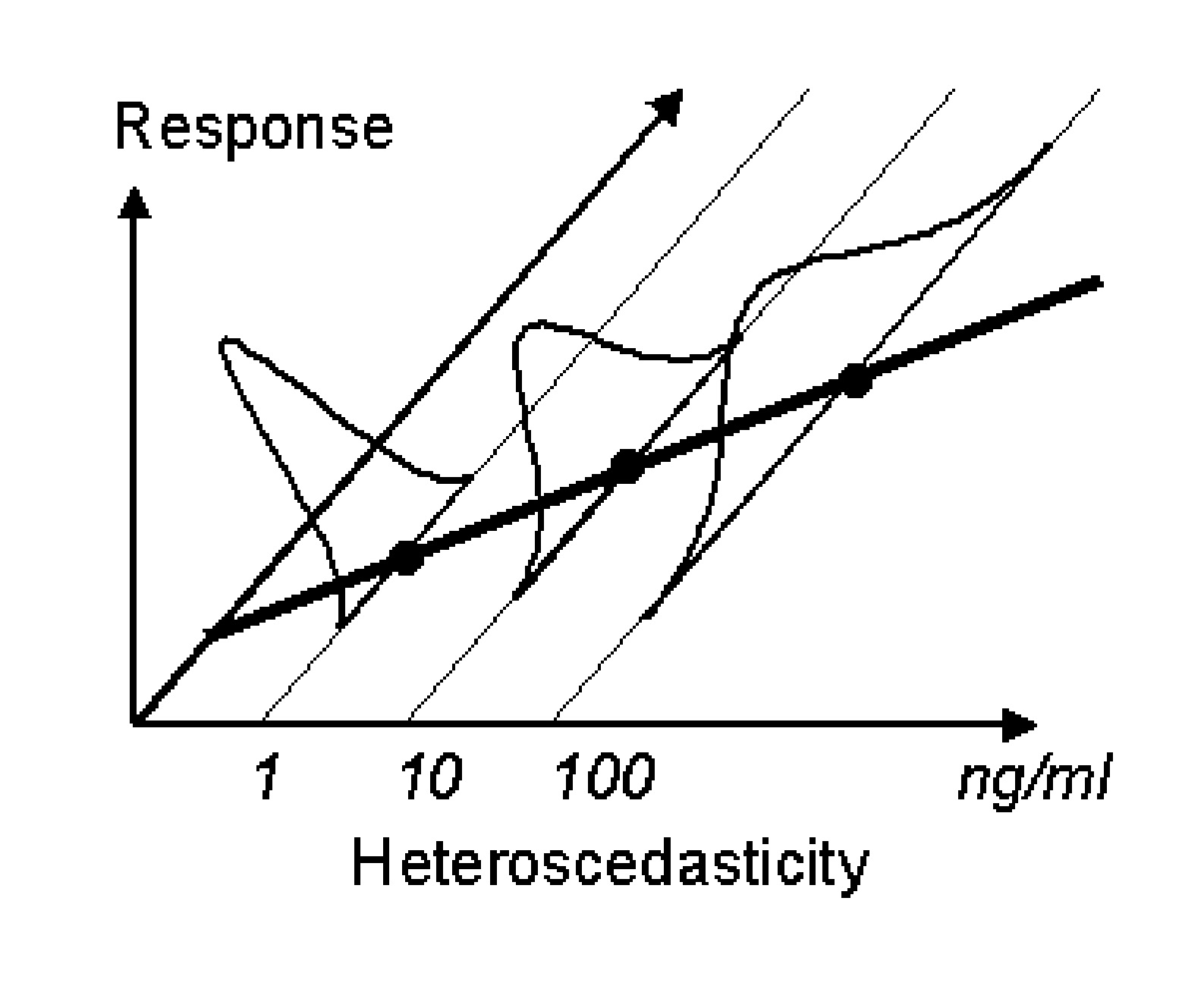
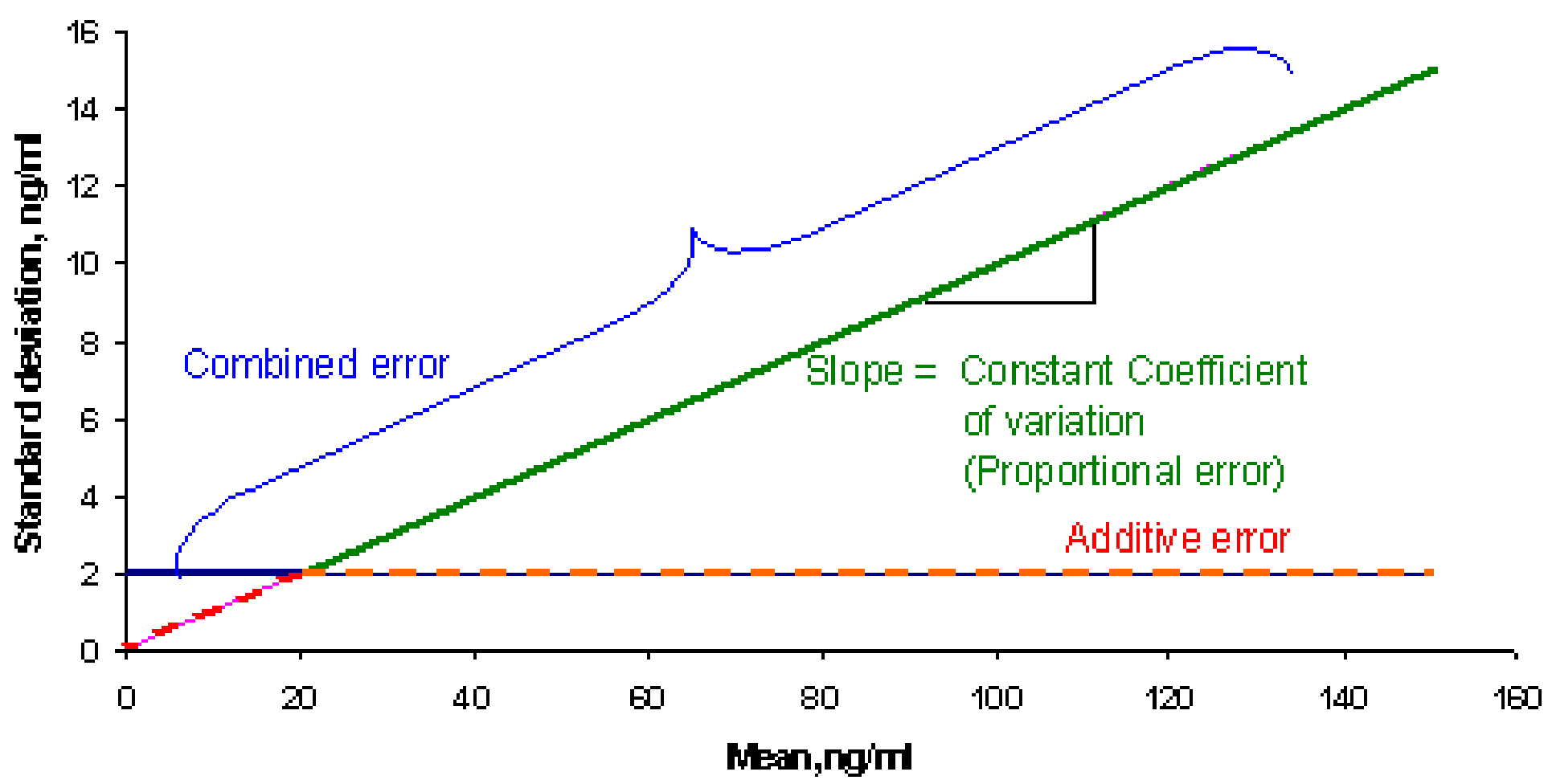
If we consider plotting the standard deviation against the mean concentration from figure 1, it would result in a line similar to the flat line shown in Figure 3 below. Similarly when the heteroscedastic standard deviations from figure 2 are plotted against means, the plot will look like the inclined line as in figure below. The flat line represents the additive or constant error component. The slope of the inclined line would be equal to the coefficient of variation. Therefore, when the error is proportional to the concentration, such an error model is called a constant coefficient of variation error model or proportional error model

Based on the above mentioned concepts, four different types of residual error models are described below.

• If the variance is assumed to be constant for all observations, then the weights are typically set to a constant value, usually 1. Such an error model is called an additive or constant error model. An additive error model is written as y_ij = y_mij + ε_ij

where

• • • y_ij = observed concentration in indiviual i at time j
    • y_mij= model (m) predicted concentrations in individual i at time j
    • ε_ij = independant, identically distributed statistical errors with ~N(0,σ²)
• Sample analyses in PK studies are normally performed using HPLC or LC-MS-MS techniques. With such analytical methods, it is observed that the precision often changes with concentrations. The experimental errors are considered to be heteroscedastic and can be written as:

  • A constant coefficient of variation (CCV) model or a proportional model
    y_ij = y_mij •(1 + ε_ij)

  • Another way of writing a CCV model is the exponential error model(approximates constant coefficient of variation)
    y_ij = y_mij •exp(ε_ij)

• In the case of PK concentrations, where wide range of concentrations are measured, the error in measurement based on the analytical method is usually a combination of additive and proportional or exponential error. Use of a combined error model would improve predictions at lower limit of assay precision where variance may be assumed a constant and a proportional error model at higher concentration range.
  • A combined error model can be written as
    y_ij = y_mij + y_mij •ε₁+ ε₂ or y_ij = y_mij•exp(ε₁)+ ε₂
• In population analysis,
  • a proportional error model could be used when the range of concentration covers more than one order of magnitude
  • an additive error model could be used when the range of concentrations are narrow

---

Covariate Model Building

An important objective of population pharmacokinetic-pharmacodynamic analyses is to discover relationships between observable covariates and individual kinetic/dynamic parameters which explain part of between subject variability (BSV/BOV).Model building exercise is performed by addition of prognostic factors / covariates such as weight, sex, age, renal function (Creatinine clearance), hepatic function, comedication, genotypes etc., in the initial model and evaluating the goodness of fit of the new model.

Importance of covariate modeling

1. In drug development process, quantitative modeling of covariates will allow one to determine whether subgroups of patients need special dosing recommendations.
2. Simulation of new trials could be performed by including the covariate information.

Identification of influential covariates

1. Primarily, identifying covariates should be based on biological plausibility.
   1. For ex., a possible dependance of drug clearance on individual creatinine clearance could be tested if a compound is known to be excreted unchanged to an appreciable extent.
   2. Another example could be the influence of comedication could be investigated if it the drug is known to induce or inhibit one of the primary metabolizing enzyme.
2. Graphical analyses of covariates
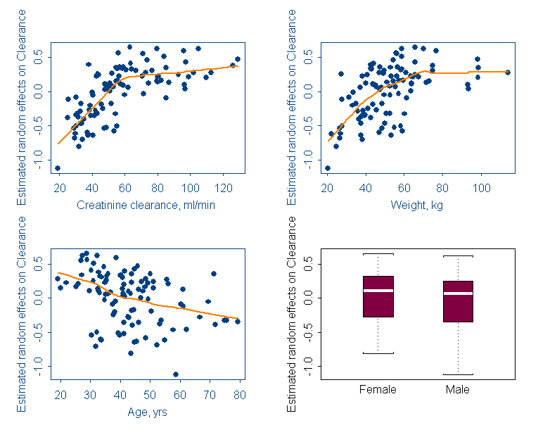
   1. Scatter plots of individual between subject variability of parameters (η_CL's, η_V's) and covariates could be checked for any trend. An example scatter plot between η's and covariates is shown below.
   2. Correlation between observed covariates, like a correlation between age and creatinine clearance is also revealed from scatter plots. In such a case, only one of a pair of correlated covariates is included in the model.

Covariate model specification

• Base model: CL_i = CL_pop • exp(η_CL)

To add effect of weight on CL, the different types of covariate models that could be used are given below.

1. Linear additive effect
   • CL_i = (CL_pop + θ•BW) •exp(η_CL)
     where
     CL_i = individual clearance
     CL_pop = Population clearance
     η_CL = random between subject variability
     θ = shift parameter describing the systematic dependance of CL on individual body weight.
2. Normalized by median weight
   • CL_i = (CL_pop + θ•BW/(Median BW)) •exp(η_CL)
3. Centered on median weight
   • CL_i = (CL_pop + θ•(BW-Median BW)) •exp(η_CL)
4. Power or allometric model
   • CL_i = (CL_pop•(BW/70)0.75) •exp(η_CL)

Hypothesis testing
Hypotheses testing on covariates identified based on physiology and graphical analyses are done by including one covariate at a time. Log-likelihood ratio test (Model selection criterion) is used to test the hypothesis and to identify significant covariates. Selection of covariates is based upon both clinical and statistical significance of covariates.

---

Evaluation of Final Parameter Estimates and Model Selection

In order to characterize that the present model is representative of the data at hand, more than one selection criteria needs to be looked at.

Following are few suggestions:

Diagnostic plots

Predicted vs. observed concentration will give you an overall sense of how well the model is doing. Weighted residuals vs. predicted concentration, residuals vs. time, and weighted residuals vs. time will also help diagnose potential errors related to the model selected and the variance structure.

Normally, the following plots are looked at:

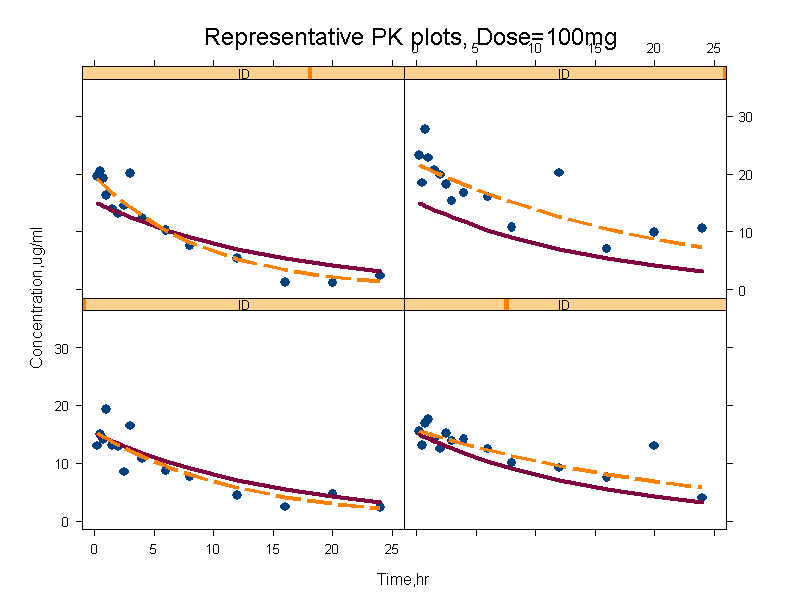
• Individual plots of observed and predicted concentration versus time. A goodness of fit plot where each individual profiles could be seen. A plot of representative individuals is shown.

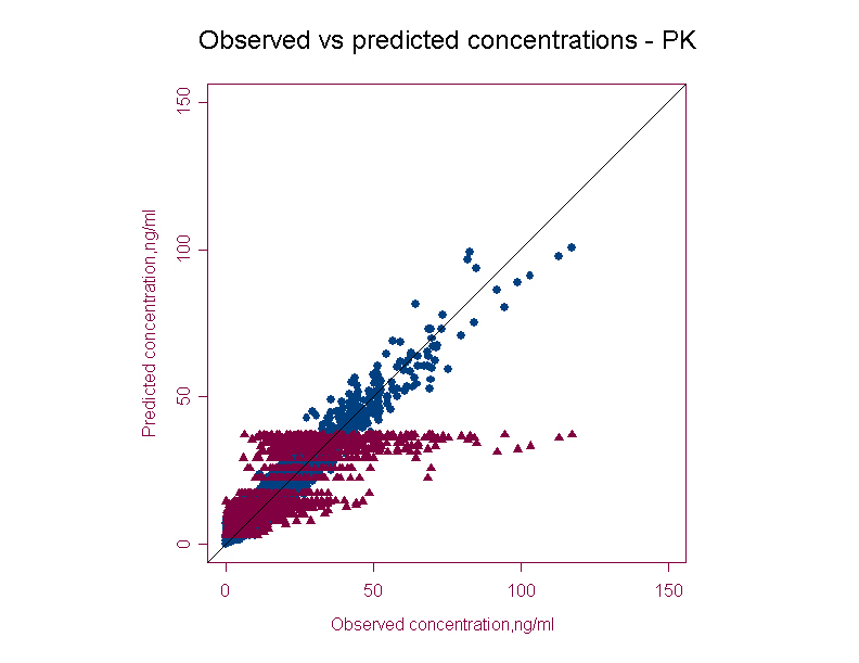
• PRED & IPRED versus DV (population predicted and individual predicted versus observed concentration)

This graph provides the overall trend in the data. Ideally the concentrations should be uniformly randomly distributed along the line of identity. Any bias seen in the population predicted plot will pinpoint exploring any covariate relationship. Individual predictions are usually better than population predictions.

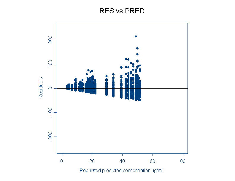
• RES vs PRED (Residuals versus population predicted)

Residuals are difference between an observations and its population predictions. This plot provides a useful picture of the residual error distribution. For a proportional error model, the residuals are cone shaped. For an additive error model the residuals are evenly distributed.

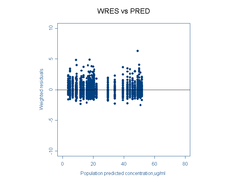
• WRES vs PRED (Weighted residuals versus population predicted)

This plot signifies whether the variability is modeled correctly or not. There should be uniform spread of the data without any trend. If any trend is observed like a S-shaped wave, then it is necessary to transform the data or use a different residual error model.

Note: Though residual plots are some of the goodness of fits plot explored, the utility of theses residual plots is not well documented.

Difference in Objective function value (DOFV)

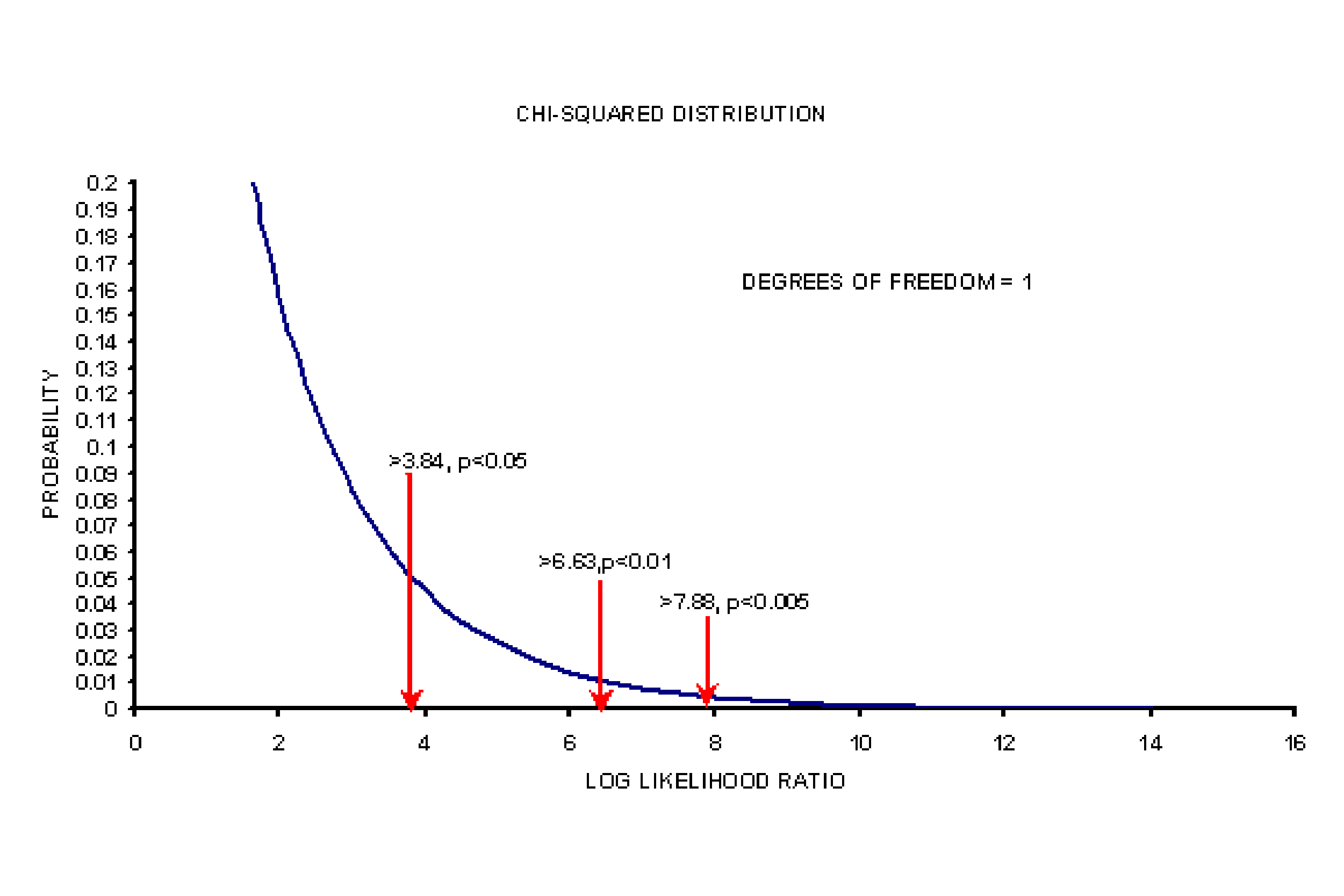
In the case of nested models (one model is a subset of other, i.e, null model (without covariates) is a subset of full model (with covariates), the difference in the objective function value or in other words, the log-likelihood ratios (LLR) are assumed to follow a chi-square distribution. The decision on choosing the null model or full model is based on the degrees of freedom (difference in number of parameters), pre-specified significance level and the critical chi-square value at that significance level and degrees of freedom.

For instance, a difference of 3.84 units in OFV between the competing models is considered significant at p < 0.05 and with one degrees of freedom.

Plot of a chi-squared distribution for one degree of freedom with critical chisquare value is shown below:

Akaike information criteria (AIC)

• AIC is used in the case of non-nested models.
• AIC = Objective function value + 2*p, where p = total number of parameters in the model (structural+error). Lower the value of AIC better the model.

Precision of the parameter estimates

The precision or the standard error of the estimate could be obtained by the modeling process and can be compared between competing models. If the standard error is large, then probably the model could be overparametrized.

---

Model Validation/Qualification

A model and its set of parameters are deemed 'qualified' to perform particular task(s) if they satisy apre-specified criteria.¹

Currently, there is no consensus on an appropriate statistical approach to qualify population PK models.Recently, there was a conference on model qualification, where various approaches and case studies were discussed. ²

FDA guidance provides different types of model validation and validation methods.

1. Gobburu,J & Marroum,P:Utilisation of pharmacokinetic-pharmacodynamic modeling and simulation in regulatory decision making.
2. ECPAG 2004